Measuring expected credit loss: Loss rate vs. Probability of default
Some time ago I published an article about calculating bad debt provision in line with IFRS 9.
Precisely speaking, it was about measuring expected credit loss using simplified approach for trade receivables – just to be on the safe side.
Since then, I keep receiving loads of questions such as:
“Why did you not use three-part formula of EAD x LGD x PD?”
Answer: It’s a great formula, but not for everybody. Read more here later in this article.
“Why don’t we apply PD (probability of default) in provisioning matrix?”
Answer: It seems you are confusing two different methods of calculating ECL, please read more below.
“What if my debtors always pay, but very late? Do I have ECL?”
Answer: In short – yes. For more explanation, read below.
So from these and other questions I can see that there is a bit of confusion about calculating ECL and therefore I want to shed some light to this topic.
How to measure expected credit loss?
There is no imperative rule in IFRS 9.
Let me stress this out LOUD:
There is NO one single method of measuring the expected credit loss prescribed by IFRS 9.
Instead, it is YOU who needs to select the approach that fits your situation in the best way.
IFRS 9 only tells you that any method you select MUST reflect the following (see IFRS 9.5.5.17):
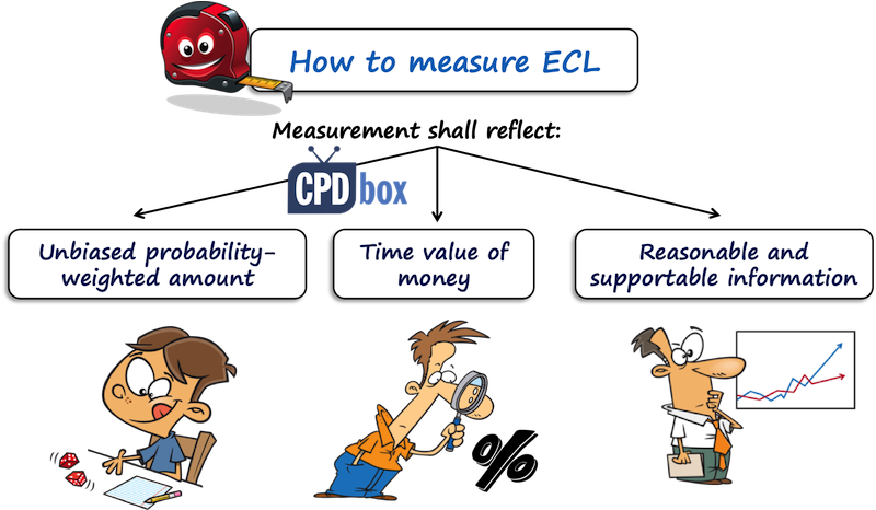
1. An unbiased and probability-weighted amount…
…to which you have arrived by assessing a range of possible outcomes.
Illustration: Imagine you have a debtor who owes you CU 1 000 000 (CU = currency unit) repayable in 2 years. There is some chance that due to economic downturn, the debtor will lose sales and as a result he would not be able to repay fully.
And, you identify 3 different outcomes: either the debtor pays you in full, or pays you just 50% on time and the rest some years later, or goes bankrupt and you lose 100%.
You need to assess each of these outcomes, how probable they are, how much you would lose in each outcome and calculate ECL.
2. The time value of money
You should discount the estimated losses to the reporting rate.
This is done because the losses can occur in more than 12 months after the reporting date.
For example – the debtor from the above illustration should repay in 2 years and let’s say that can go bankrupt in 2 years.
Now, at the reporting date, when no payments from that debtor are due, you can still have expected credit loss because you might expect that the debtor will not repay anything in 2 years.
But, as the loss is expected in 2 years, it is necessary to bring it down to present value, because otherwise the loss would be greater than the carrying amount of a loan itself (as it IS in present value).
Also, you can incur the loss even if the debtor pays you in full, but later than expected, exactly due to time value of money.
One reader asked me a question:
“We trade with our government and have trade receivables towards them. The government always pays us, but the payment arrives 20-24 months later than due. Do we have some credit loss here?”
The answer is – YES, you do, exactly because the time value of money.
If the payments arrive a few months later, then you can probably ignore the time value of money as the period between the arrival of payment and due date is less than 1 year and thus the effect of discounting would not be material.
But, this is not the case when the payments arrive almost 2 years after due date.
Reasonable and supportable information…
…available without undue cost or effort at the reporting date about past events, current conditions and forecasts of future economic conditions.
Hmmm, I get LOADS of questions on this one.
How do we get loss rates since we are a new entity and have no historical data?
How do we incorporate forecasts if we have no information on them?
Well, let me tell you that sometimes you need to look at external sources of information and simply BUY the data.
Let’s say you are a new retail operator and have no history of payment discipline of your customers.
Thus you cannot calculate historical loss rates as I have done in this example.
OK, then you might need to apply the alternative approach.
For example – use the information from similar entities operating in similar industry in similar economic environment.
You can buy this info from credit bureaus, credit rating agencies, economical statistics prepared by central banks… you need to be a bit open-minded here and look for what is available in your country.
And remember – the standard does not say that the reasonable and supportable information must be obtained with NO cost at all.
It says “without undue cost and effort”, so yes, IFRS 9 practically says that you might incur some cost to get the info.
What are the most common methods of measuring ECL?
Here we are getting to the clarification of all those loss rates, probability of default rates, “three-part formula” and other terms related to measuring ECL.
Basically (that’s what most banks and other entities do), there are just two most popular methods:
- Loss rate approach,
- Probability of default approach
Again, this is NOT imperative.
If you can come up with a different method – fine, apply it, but remember it must meet the three criteria set by IFRS 9 as described above.
Now let’s bring some clarity to these methods and illustrate them a bit.
I. Probability of default approach
Here, three elements enter into the calculation of expected credit loss:
- Probability of default (PD) – this is the likelihood that your debtor will default on its debts (goes bankrupt or so) within certain period (12 months for loans in Stage 1 and life-time for other loans).
- Loss given default (LGD) – this is the percentage that you can lose when the debtor defaults.
- Exposure at default (EAD) – this is the amount that the debtor owes you at the time of default.
The formula for calculating ECL using this method is here:

Let me illustrate this method a bit.
Example: Probability of default approach
Let’s say that you have a debtor that owes you 1 000 CU repayable in 1 year. The debtor has severe financial troubles and your lawyers estimate that there is 20% chance of going bankrupt. If the debtor goes bankrupt, you would lose 70% of the amount he owes you. You lose nothing when there is no bankruptcy.
In this short example:
- PD = 20%;
- LGD = 70%;
- EAD = 1 000 CU.
Thus, the expected credit loss is 20% x 70% x CU 1 000 = CU 140.
Sure, I ignored both of:
- The stage of this loan – because the remaining life of the loan is 1 year and thus 12-month ECL = lifetime ECL.; and
- The time value of money – because the loan is repayable in 1 year and it is likely that time value of money is not material.
In reality, you need to take care about all of these things.
In fact, this calculation takes TWO outcomes in consideration:
- Loss with 20% probability; and
- No loss with 80% probability.
The full formula is therefore:
- 20% (PD) x 70% (LGD) x 1 000 (EAD); PLUS
- 80% (=probability of NO default = 100% – PD) x 0% (zero loss) x 1 000 (EAD)
- = 140.
I am just adding it here because you might have some loss even in “no default” situation due to late payments (time value of money!).
You can also see the example illustrating this method on undocumented intercompany loan here.
Pros and cons of PD method
This method is preferred by banks and financial institutions, because they have large portfolios of loans and great internal credit rating system in place.
Also, this method is compatible with Basel capital framework requirements, so the banks need to make a few adjustments to make it in line with both Basel and IFRS 9, too.
I would also say that probabilities of default include certain forward-looking insights in them and are not based purely on past statistics, thus they are OK with IFRS 9.
However, for trade receivables and other financial assets where you can apply simplified approach, this is not very convenient, because of challenges involved in getting the necessary information.
It is quite difficult to develop internal statistical models for getting PDs and other information.
Therefore, most companies use the second approach for their trade receivables and other financial assets where simplified model is applied: loss rate model.
II. Loss rate approach
Here, you do NOT need any probability of default (PD) and other details.
The two things that you need are:
- To get historical loss rates of your own financial assets.
You need to develop some statistics of amounts never paid by your customers (write-offs, or losses). I showed you how to do it here in this article with the example. - To adjust them by forward-looking information.
This is the difficult part. If the economic and other environment did not change, then you are all OK, but when there are economic changes (recession, new competitors, new laws), then you need to examine those changes, estimate their impact on your receivables and incorporate it in the loss rates.
I also showed you the example in this article.
When you are using so called “provision matrix”, you are applying loss rate approach in fact.
I am not bringing any illustration of this method here, because it is fully and in detail showed here.
Pros and cons of loss rate approach
This method is quite simple, because you can always calculate the loss rates of your receivables (if you are a new entity, then read above for guidance).
However, there are two drawbacks of this method:
- Forward-looking information: oh yes, I repeat: loss rates as such reflect only past information, i.e. what has already happened. You have to make an adjustment for the information about the future performance of your portfolio.
- Time value of money: If you have trade receivables or other financial assets with repayment date of less than 12 months and you assume that all amounts unpaid within 12 months are lost, then you can ignore discounting. But, if you have financial assets with longer maturity periods, or your debtors pay you in more than 12 months after the maturity date, then you need to incorporate time value of money as well.
Any questions? Please let me know in the comments below this article. Thank you!
JOIN OUR FREE NEWSLETTER AND GET
report "Top 7 IFRS Mistakes" + free IFRS mini-course
Please check your inbox to confirm your subscription.
61 Comments
Leave a Reply


Hi Silvia
What would be the impact of actual bad debts written off during the year on the calculation of expected credit losses?
Naturally, you would need to take this number into account when assessing your historical PD.
Hi Silvia
Could you please advise if we can use LGD and PDs in simplified approach? The reference is my client having long term recievables from customers. They are using simplified approach but incorporating the element of LGD and PDs in this approach. In your articles and the IFRS 9 publications, I have never came across any such situations where these elements are used in the simplified approach. Could you please provide a reference to the standards too in your reply.
Hi Silvia
How can I relate the figure of GDP and inflation to my PD% in ECl model to discount the PD % at an appropriate rate, noting that I have the historical and forecasted figures for GDP and inflation and also I use the simplified approach in determining ECL value.
Well, that is the task of creating suitable model that reveals how the performance of your portfolio of receivables correlates with these factors, such as inflation or GDP. It can be different for each company depending on the industry, structure of customers, etc.
Dear Silvia
Do I need In simplified approach to take in my consideration the inflation rate ??
Hi Silvia
Is ECL needed in a situation where an entity has receivables due from its shareholders. These receivables relate to unpaid share capital. The entity is still has not commenced operations as such the shareholders would be paying at later date in future.
Thank you.
Hi Dan, yes, it is, sorry, because ECL is about the asset side regardless the way how that asset was created. However, in most cases, ECL on this type of receivables is close to zero.
Thank you
Hi Silvia,
Can you help me about how to calculate percentage of PD and LPD?
Thanks.
Dear Silvia
First of all thank you very much for your effort.
I need ask you about simplified approach
In the event that I have customers who are always late in payment for a period of up to two years, but in the end they pay in full,
how do I calculate the time value of money.
If I make a provision of 100% after one year of the debt and after another year I get the full value of the overdue bills, do I close this provision in a profit account?
Thank you in advance
Hi Hany, general view is that unless you charge late payment interest or so, the effective interest rate on trade receivables is usually zero, so there is no effect on discounting (time value of money). After all, that’s why it is possible to use simplified approach when there is no significant financing component (i.e. interest).
To the second part of your question – when you make an individual provision to the specific receivable, then of course you need to reverse it when the receivable is collected. If you are using collective approach (like provision matrix), that would solve itself by updating your provision automatically. S.
Thank you for your response
last question
about simplified approach can I make it exceed 12 month (My matrix)
for example
0-30 1%
30-60 5%
60-90 8%
90-180 20%
180-270 40%
270-365 60%
365-547 80%
365-730 100%
In order to comply with the nature of my collection
Does the standard allow this?
Sure, if that corresponds with your historical experience and forward looking information.
Thank you for your support
I appreciated
ECL model is more focusing on bringing the bad debt provision when it is due rather when it is incurred and we can provide loss right from day 1 rather waiting for actual bad debt happens.
Suresh, you posted multiple comments below my articles with the sole purpose of advertising your website. Most of these comments bring no further value to the readers, just rinse and repeat what was already written/said elsewhere (on this site). Deleted, including your ads. Next time please post comments with the purpose of helping people and not for the sake of promoting your site and services.
Hi Silvia, it is first time to comment and I’m really appreciate your great efforts.
I have a question as I’m an auditor and when I was auditing Accounts Rec for one customer he told me that all outstanding balance at the year end has already been collected subsequently and he showed me evidence for proof of receipt. In this case do I still need to calculate ECL. The customer told me not to do so.
Hi Khaled, thank you. It depends. The truth is that you should take the information valid at the reporting date into account, and post-year-end collection clearly surpasses that, but we can well say that this collection can be evidence of the situation or circumstances existing at the reporting date. So, let’s say your client was in a good shape at the year-end and paid after the reporting date. This payment can be evidence of that good shape existing at the reporting date. However, let’s say your client had financial difficulties and after the year-end, it received an unexpected government support in form of cash and paid out of this support. Then it is evidence of bad financial situation at the reporting date and I would definitely provide for ECL to reflect that. Again, no black or white, you have to assess individually what the situation was.
Hi Silvia
Can I conclude that in simplified approach that I am only calculating loss rate so I shouldn’t calculate PD & LGD
Hello
Your article is very informative, I am trying to calculate ECL on Unbilled revenue and Account receivable from government ( There is no risk of default with the government in my situation), However government pay very late like around after one or two years as per the discussion above i belive that i only have to take the impacts for time value of money for the calculation, but my question is that what interest rate i should use and what will be the equation( formulae) for the calculation of ECL in this senario
I am looking forward for your positive response as soon as it is possible as i have deadline to complete this task
Thanks
hi silvia,
since 2015 i follow your all post either video or other.
however, i really need your help to guide us how to calculate ECL in our own entity where we will start applying FULL IFRS version instead of SMEs IFRS version .?
thanks in advance and Regards.
Hi, Amazing Article.
Question is, using the Probability of Default approach, how do you develop a model to calculate probability of default in a bank
Hello Silvia,
Great simplification!.
In exposure of default, can we consider only unsecured portion of debt instead of total debt?
How do we assess for related party receivables when there is a outstanding payable for the same related party which in excess of the receivable balance, in this case, do we have to assess ECL for the receivable portion..??
Hi
I was calculating ECL on related party loans, and i discounted future cashflows using a discount rate equal to commercial interest lending rate. Then the difference between the present value of the loan and discounted future cashflows is my ECL.
The cashflows i used was based on the loan terms, adjusted against management cashflow forecasts.
Is the method appropriate and adequate?
HI Silvia,
My question is what if the Loan has a credit enhancement say a collateral, and that collateral’s realizable value fully covers the EAD or outstanding balance. Would that automatically mean that LGD is zero? Consequently, if the PD LGD EAD model is used under the General Approach, would that mean that ECL for fully collateralized loans is zero?
Appreciate if you can shed some light on this.
Thank you
Hi Derrick,
while collateral affects the amount of LGD (not EAD and not PD – to clarify to other readers), I would not say that it reduces your LGD to zero even if the loan is fully collateralized. The reason is that loss arises also when the payments due are collected with time delay, due to time value of money, and I’m quite sure that it would take some time and expenses to get the loan repaid by means of collateral. Also, another thing is to evaluate collateral, especially in today’s situation and if a collateral is some property (or other assets). Because, let’s say that the market crashes and the value of properties declines sharply, then your collateral may NOT cover the full loan outstanding and again, your LGD (and consequently ECL) would not be zero. S.
Hi Silvia, thank you for the information, just a some clarity do we need to keep calculating the default rate yearly if say i calculated it for 2019 in 2020 is should still calculate default rate and apply the forward looking rate?
Hi Sylvia!,
In your IFRS kit, ECL=credit loss X default risk. Whereas, in the article above the formula is slightly different. Kindly explain if they mean the same thing and how?
Thanks
Hi Surabhi, it is not different. Credit loss is in fact LGDxEAD, so LGDxEADxPD = credit loss xdefault risk. Please bear in mind that there are more approaches to calculate ECL 🙂 you don’t need to use LGD at all.
Thank you so much!
Hi silvia
thank you for such an informative article. i’m wondering about the 3 stages in general approach and its differences from the previous standard (IAS 39). i wish you can talk about this in the next article. thank you
Hi Sylvia,
At formula level, both under IAS 39 and IFRS 9, most of the time loan allowance is calculated as EAD x PD x LGD. So which variables would change due to adoption of IFRS 9.
My understanding is that the change from incurred loss to expected loss will be reflected in LGD, whereas there won’t be major change in EAD or PD due to adoption of IFRS 9.
Is this correct?
Thanks.
Thank you for such an informative article. However am having a challenge computing PD. My company is a security brokerage firm having very few receivables. I would appreciate if you assist me get to know how to calculate PD in order to arrive at ECL.
Hi Sylvia,
Thanks for your articles about different IFRS statements . It helps us a lot in order not to forget our IFRS knowledge and help us to use it, whenever it is needed.
Best regards
Hi Sylvia,
It would be nice to see your article on calculation of impairment allowance by banks (using PD, LGD and EAD)
Thank you Silivia
You’re super faster !
I’ve gone through many articles where IFRS suggest to consider 2-5 years period. Reason being last year data would be so new while ignoring industry trend. Example last year company has put extra effort to collect or that period resulted with less sales or government and the industry allocated limited budget for development ( medical equipment industry). So I would rather suggest to take 3 years period and assess the loss every year and average plus adjust with the forward looking factors. Then apply to current year closing receivable aging .
2nd thing is I’m not getting how to adjust with FV/ PV .
Thanks for your support
Yes, that is possible, too. There are many different considerations that you need to take into account. However, if the loss rates in year 2007 were low and then in 2008 the financial crisis came and everything went down, it would not be appropriate to include the rates of 2007 into the calculations. Hence you know what I mean by considering 🙂
Hi Silvia,
Can you please develop a provision matrix and demonstrate?
Assume in 2016 I have loss $1000 and 2017 $500 and 2018 $2500. So do I have to calculate loss rate every year and I get the Average against selected aging balances ? Then I adjust the forward info and apply the adjusted loss rates to 2019 aging?
But how to incorporate present value into this calculation?
Thanks
Hi Mohamed, I DID develop a provision matrix and I linked a few times to it in this article, but here it is again, just for you – CLICK HERE to see the article with the exact approach of how I developed provision matrix.
Indeed I’ve gone through earlier matrix, what my question is that , when I take more than 1 year analysis I need to take loss rate every year and then take average right?
How to apply PV ?
Thanks
Hi Mohamed, I don’t think this is appropriate – you should make your assessment. The thing is that the newer data are closer to the reporting period and say more about recent situation rather than data older than 1 year. I would better update loss rate calculation each year based on new data and adjust it for forward looking info.
It is better to go through, account by account; and writeoff those with very remote likelihood; and provide 100% (full impairment) for other long outstandings. Which in substance both are the same. However, in many companies (especially, public enterprises); they have used this opportunity of IFRS conversion to writeoff such balances after approval by their board/another body. And, as Silvia indicated; the standard does not prohibit a continuous contra account (allowance for provision).
Hi Kiros, thank you for the comment. Well, IFRS 9 is quite sticky in derecognition of financial assets – i.e. in write-offs. It specifically says that you can derecognize only when the contractual rights from the asset expire (or transfers assets that do qualify for derecognition). The question is that when there is very remote likelihood of collecting, your contractual rights from the receivables expired – they are probably still there (however, check your legislation related to that matter, it could be different). And yes, you can go account by account – that is the individual assessment not mentioned in this article. However, you can apply those 2 methods on assessing individual debtors, too.
Well kiros you know its very remote to make write offs in public organizations,you can’t most of the time. We know the concept but not applicable as you know. By the way holding 100% provision has also big problem in profit performance reports.I asked Ms.Silivia’s comment just to get her remark for knowledge.
Really most of them are government organizations still operational,as the shipping company also belongs to government it seems no willingness to pay. Am just asking you because am member in the IFRS implementation team to provide them a better suggestion for this big out standings. Also 100% loss provision implementation is so scary 🙂
Also don’t you think holding 100% provisions may affect profitability of the company,What about past years performances also,profit reports?
Thank you very much for your reply. I am thinking its not normal to hold continuous provisions every year for out standings that have no decisions,i don;t know Silvia
Well then you really do need to assess whether the asset (receivable) meets the conditions of derecognition under IFRS 9. For example – is the debtor still in operations? Or was it liquidated? etc.
Hi Silvia,its great article. Let me ask you to clarify me an issue if you allow.
I am working in shipping company in Ethiopia. currently we are in processes to adopt IFRS to prepare our financial statements. We have big outstanding balances of trade receivables,due dates passed more than 10 years . There is no practice of making write offs for held provisions of bad debts,every year the bad debt account increases. To my understanding IFRS doesn’t allow holding continuous provisions. Its clear that we should perform ECL as per IFRS 9. how do we handle such issues. I feel the simplified approach is the right method to implement. what do you think?
Hi Rahel, well, you need to recognize a provision of 100% – I doubt that you would ever receive anything after 10 years. You cannot derecognize asset before the contractual rights from it expire (see IFRS 9.3.2.3). Anyway, where does the information about “not holding continuous provisions under IFRS” come from?
Hi Silvia, Thank you for all the informative articles you are providing. In the case of Rahel, and if she recognizes 100% of the amount and due to certain circumstances she manages to collect a portion of the receivables, what is the subsequent measurement in that case, Recognize profit in P&L? and if so of what sort.
Thank you
Yes, you need to reverse the impairment loss on the receivables, as a “reversal of impairment loss”, basically in the same line item (or below) as the recognition of the impairment loss on financial assets.
Thanks Silvia
The calculation and assessment of ECL takes place on reporting date and cannot include information after the reporting period which could not possibly be known as at that date. Hindsight information cannot be used. Therefore, the fact that the debtor repaid 12 months later for example cannot affect the calculation of ECL. ECL should be assessed and calculated as at the reporting date and should be based both on historic and forecast information that could be reasonably assessed usign the knowledge in hand at the reporting date. Hindsight info cannot be part of that assessment.
Hi Andreas, thanks for the comment and I agree. The fact that I mentioned debtors not repaying within 12 months relates to the calculation of historical loss rates, not to the application of hindsight. To make it totally clear: Let’s say you are calculating your past loss rates and there were no losses in the past – i.e. everyone paid. But, significant debtor always paid 16-20 months later than due date. Thus there was a loss due to time value of money and you should incorporate that historical loss when making ECL on the current balance. This is not hindsight at all because you are using past information about past late payments of the debtor.
Hi Silva,
Thank you for the valuable insights.
Is it possible to incorporate TVM in determining your loss rate?
We have a portfolio of debtors that usually pay us less than 60 days. However certain balances are paid after 210 days. As the customers have shown in the past to settle their accounts. How loss exposure is due to time value of money. We have incorporated a time value of loss factor in the determining the ECL.
Can the time value of money only be taken into account after determining the ECL. Or can the time value of money been included in your historical loss rate?
Hi, Silvia,
Great article and many thanks.
Eventually, if we know that client subsequently fully paid his outstanding amount either in 2, or 4 or 8 months after year end should i still apply ECL?
At the end of the day, we show a picture of the accounts as at 31.12.XX. At that time i know that the client will pay 100? (assume no history of bad debts).
What i see it is all a matter of judgment.
Regards,
Marios
Hi Marios,
as I have written in this article – if the client pays late, you still have some ECL due to time value of money. However, when the payments do not arrive later than 12 months after the end of the reporting period, the ECL will be probably not material. S.