
How to calculate bad debt provision under IFRS 9
Last update: 2023
If you have a large portfolio of trade receivables, then you face the same issue over and over again:
How to calculate bad debt provision to these receivables?
When I worked as an auditor, I used to discuss this issue with my colleagues very frequently.
Everyone of them agreed that yes, there is always some bad debt hidden among “healthy” receivables and it’s necessary to recognize some provision for that.
However, everyone had a different opinion on how to do it.
The most common approach was, to my surprise and disagreement, to create a provision in a few steps:
- Analyze receivables at the reporting date and sort them according to their aging structure
- Apply certain percentages of provision to the individual aging groups
Sounds easy, right?
In most cases, auditors applied something like 2% to trade receivables within maturity, 10% to trade receivables that were 1-30 days overdue… 100% to receivables more than 360 days overdue.
It always amazed me.
How the hell do you know that this particular company will suffer 10% credit loss on receivables that are 1-30 days overdue???
For me, it always seemed that these numbers were made out of thin air.
It was long time before IFRS 9 was adopted.
Now, luckily, IFRS 9 tells us how to create bad debt provision for trade receivables and how to get these percentages.
In this article, I’d like to explain this methodology and illustrate it on a simple example.
What do the rules in IFRS 9 say?
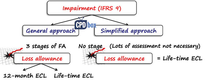
IFRS 9 requires you to recognize the impairment of financial assets in the amount of expected credit loss.
In fact, there are 2 approaches for doing so:
- General approach
In general approach, there are 3 stages of a financial asset and you should recognize the impairment loss depending on the stage of a financial asset in question.Thus, the impairment loss is either in the amount of a 12-month expected credit loss (ECL) or a lifetime expected credit loss (ECL).You can read more about the general approach here.There are a lot of implementation troubles and challenges, for example:
- How do you determine in which stage the financial asset is?
- How do you determine when the credit risk in some financial asset has significantly increased?
- How do you calculate 12-month ECL and lifetime ECL?
- How do you get and update your inputs into the ECL calculations?
Therefore, IFRS 9 permits an alternative for some type of financial assets:
- Simplified approach
In simplified approach, you don’t have to determine the stage of a financial asset because the impairment loss is measured at lifetime ECL for all assets.This is great news because lots of troubles simply disappear.
However, let me warn you that the simplified approach is not for everybody and even if it’s simplified, you still need to make some calculations and effort.
Who can apply simplified approach?
OK, that’s not the best question in the world, because everybody can apply simplified approach.
Type of financial asset is more important here.
You have to apply simplified approach for:
- Trade receivables WITHOUT significant financing component, and
- Contract assets under IFRS 15 WITHOUT significant financing component
For these two types of assets you have no choice – just apply simplified approach.
On top of that, you can make a choice for:
- Trade receivables WITH significant financing component,
- Contract assets under IFRS 15 WITH significant financing component, and
- Lease receivables (IAS 17 or IFRS 16)
For these three types of financial assets, you can apply either simplified approach or general approach.
Can one entity apply both models?
Yes, of course – but not to the same type of financial asset.
Take a bank, for example.
Banks usually provide lots of loans and under IFRS 9, they have to apply general models to calculate impairment loss for loans.
But occasionally, banks can have other financial assets, too.
For example, they may rent redundant offices and have lease receivables.
Or, they can provide advisory services and charge fees for that – thus they can have typical trade receivables.
For these types of assets, the same bank can apply simplified approach.
How to apply simplified approach?
As written above, under simplified approach, you measure impairment loss as lifetime expected credit loss.
IFRS 9 permits using a few practical expedients and one of them is a provision matrix.
What is a provision matrix?
Simply said, it is a calculation of the impairment loss based on the default rate percentage applied to the group of financial assets.
Here, we have 2 important elements:
- Group of financial assets
- Default rates
Let’s break it down.
How to group the financial assets?
When you are using provision matrix for simplification, you still need to be as close to reality as possible.
Therefore, before applying any loss rates, you should group your financial assets first.
Segment them.
The reason is that all trade receivables do not necessarily share the same characteristics and therefore, it would not be reasonable to put them into the same pocket.
How to group them?
It depends on what factors affect the repayment of your receivables.
Maybe you noted that your retail customers (individuals) are less reliable and slower in payments than your business customers (companies).
Therefore, your segments or groups would naturally be retail customers and business customers.
Or, maybe you sell in a few geographical regions and you noted that customers from the capital city pay more reliably than customers in the rural areas (maybe it has something to do with unemployment rate…)
So, your segments would be customers from cities and customers from countryside.
I think you get the point – you should select the grouping of your trade receivables (or other financial assets in questions) depending on your circumstances.
Just a few suggestions for segmenting:
- By product type;
- By geographical region;
- By currency;
- By customer rating;
- By dealer type or sales channel;
etc.
The important point here is that the customers within one group should have the same or similar loss patterns.
How to get the default rates?
Remember – do NOT just trump the default rates up, just like auditors from the intro of this article.
You should really calculate them based on your own data.
IFRS 9 says that you should:
- Derive the default rates from your own historical credit loss experience; and
- Adjust them for forward-looking information.
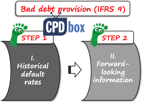
Historical default rates
First, you need to analyze the historical credit losses.
How?
You should take the appropriate period of time and analyze which portion of trade receivables created during that period went default.
Just be careful when selecting the appropriate period.
It should not be too short in order to make sense and it also should not be to long because market changes quickly and long period might incorporate market effects that are no longer valid.
I recommend selecting one or two years.
Then you are going to select the time buckets, or periods when the receivables were paid.
Finally, you would calculate the default rate for each bucket.
No worries if this seems too unclear – you can find the illustrative example below.
Forward-looking information
Once you have your historical default rates, you need to adjust them by the forward-looking information.
What is it?
They are all information that could affect the credit losses in the future, for example macroeconomic forecasts of unemployment, housing prices, etc.
You should adjust historical default rates for the information that is relevant for your financial assets.
For example, let’s say the telecom company has 2 segments of receivables:
- Retail customers, or individuals and for this group, unemployment rates are important factor affecting the payment rate.
If unemployment goes up, the credit quality of trade receivables to retail customers worsens. - Business customers: for this group, GDP (gross domestic product) and inflation rate are important factors in this particular country.
How to incorporate the forward-looking information?
When there is a linear relationship between the macroeconomic factor (i.e. unemployment rate) and the input (i.e. increase/decrease in collection of receivables), then the incorporation is quite simple.
In this case, you need to observe what effect has the change in the parameter on your default rates and make simple adjustment (see illustration below).
However, when the relationship is not linear, then the adjustment might require some modeling using either Monte Carlo simulation or other similar methods.
Example: Impairment of trade receivables under IFRS 9
ABC wants to calculate the impairment loss of its trade receivables as of 31 December 20X1. ABC’s policy is to give 30 days for the repayment of receivables.
Note: This is an important point – 30 days credit period means that these receivables have NO significant financing component and therefore, you don’t have to worry about the present values.
The aging structure of trade receivables as of 31 December 20X1 is as follows:
| Days after issuing invoice | Amount outstanding |
|---|---|
| Within maturity (0-30 days) | 800 |
| 31-60 days | 350 |
| 61-180 days | 280 |
| 180-360 days | 170 |
| > 360 days | 100 |
| Total | 1 700 |
ABC decided to apply the simplified approach in line with IFRS 9 and calculate impairment loss as lifetime expected credit loss.
As a practical expedient, ABC decided to use the provision matrix.
First, ABC needs to calculate historical default rates.
In order to have sufficient historical data, ABC selected the period of 1 year from 1 January 20X0 to 31 December 20X0.
During this period, ABC generated sales of CU 20 000, all on credit.
Then, we can split the whole analysis process into a few steps.
Step 1: Analyze the collection of receivables by the time buckets
ABC needs to analyze when the receivables were paid and sort them out into table based on number of days from creation of invoice until the collection of the receivable:
| When paid? | Paid amount | Paid amount (cumulative) | Unpaid amount |
|---|---|---|---|
| Within maturity (0-30 days) | 7 500 | 7 500 | 12 500 |
| 31-60 days | 6 800 | 14 300 | 5 700 |
| 61-180 days | 3 000 | 17 300 | 2 700 |
| 180-360 days | 2 200 | 19 500 | 500 |
| > 360 days | 500 = write-off | 19 500 | 500 = write-off |
| Total | 20 000 | n/a | n/a |
Notes:
- The amount of CU 500 in the column “Paid amount” for > 360 days represents in fact defaulted, unpaid amount.
- Paid amount cumulative is calculated as paid amount in certain time bucket plus paid amount in the previous bucket, i.e. cumulative paid amount in 31-60 days is calculated as 6 800+7 500. The exception is > 360 days – here, we can’t include CU 500 because it is not paid.
- Unpaid amount in the last column = total of 20 000 less cumulative paid amount.
Step 2: Calculate the historical loss rates
Then, ABC can calculate the historical default loss rates as the loss amount of CU 500 divided by the amount unpaid (outstanding) at the end of each time bucket:
| When paid? | Unpaid amount | Loss | Default rate |
|---|---|---|---|
| Within maturity (0-30 days) | 20 000 | 500 | 2.5% |
| 31-60 days | 12 500 | 500 | 4.0% |
| 61-180 days | 5 700 | 500 | 8.8% |
| 180-360 days | 2 700 | 500 | 18.5% |
| > 360 days | 500 | 500 | 100.0% |
Note: Default rate = loss divided by the unpaid amount.
Here you might note that data shifted a bit.
Unpaid amount for “within maturity” row amounting to CU 12 500 is now in the “31-60 days” row.
That’s OK because we are calculating amounts that fell into certain time bucket – that is, in the beginning of that bucket, not at its end.
So, in “within maturity” bucket, ABC created CU 20 000 of trade receivables; in “31-60 days” bucket, ABC created CU 12 500, etc.
Also, why did we apply the loss of CU 500 to all buckets?
The reason is that all receivables that were written off (CU 500) were in each stage over their life.
For example, all written off receivables amounting to CU 500 were current (within maturity), or within those CU 20 000 and therefore we can say that the loss generated during 20X0 (tested period) is 500/20 000.
The same applies for any other time bucket.
Now, we are not done yet.
We have only calculated the historical loss or default rates.
We still need to incorporate the forward-looking information.
Step 3: Incorporate forward-looking information
This is more difficult, but let me just outline one very simple approach.
Let’s say that ABC’s credit losses show almost linear relationship with unemployment rates.
Please note that “unemployment rate” is NOT a prescription for you – you should find your own macroeconomic factors that could affect your credit losses.
And, let’s say that the statistical office in ABC’s country assumes that unemployment rate will go up from 5% to 6% in 20X2.
ABC’s experience is that when unemployment rate increases by 1%, it triggers the increase in default losses by 10% (note – you should be able to prove that).
Therefore, ABC may reasonably assume that the loss of CU 500 can increase by 10% because of the increase in the unemployment rate – that is, to CU 550.
Thus, the calculation of loss (default) rates adjusted by forward-looking information is as follows:
| When paid? | Unpaid amount | Loss | Default rate |
|---|---|---|---|
| Within maturity (0-30 days) | 20 000 | 550 | 2.75% |
| 31-60 days | 12 500 | 550 | 4.40% |
| 61-180 days | 5 700 | 550 | 9.60% |
| 180-360 days | 2 700 | 550 | 20.40% |
Step 4: Apply the loss rates to the current trade receivables portfolio
And finally, coming to the end of this exercise, let’s apply these loss rates to actual portfolio of trade receivables as of 31 December 20X1:
| Days after issuing invoice | Amounts outstanding | Loss rate | Expected credit loss |
|---|---|---|---|
| Within maturity (0-30 days) | 800 | 2.75% | 22.0 |
| 31-60 days | 350 | 4.40% | 15.4 |
| 61-180 days | 280 | 9.60% | 26.9 |
| 180-360 days | 170 | 20.40% | 34.7 |
| > 360 days | 100 | 100.00% | 100 |
| Total | 1 700 | n/a | 199.0 |
Done.
ABC can recognize the impairment loss on trade receivables as
- Debit P/L Impairment loss on trade receivables: CU 199
- Credit Trade receivables – adjustment account: CU 199
Note: this journal entry assumes that the previous balance of the loss allowance was 0. If there was a balance, then ABC recognized just a difference to bring the loss allowance to CU 199.
Further reading
If you wish to dig deeper in the topic, here are a few articles that I recommend reading:
- How new impairment rules in IFRS 9 can affect you
- Measurement of ECL: probability of default vs loss rate approach – learn about two most common methods applied when measuring ECL, their pros and cons and illustrative examples
- How to measure probability of default – this article describes a few methods of measuring probability of default (PD) and contains my personal recommendation for external help if you need (discounts for CPDbox subscribers and readers)
- Expected credit loss on intercompany loans – learn to apply the newest ECL model
- Example: ECL model on interest-free on-demand loan
- How to calculate the impairment loss on intercompany loans?
Also, I would like to point you to our course “ECL for Accountants”, where you will learn how to apply ECL on trade receivables in much greater detail.
Any questions? Please let me know in the comments below this article. Thank you!
JOIN OUR FREE NEWSLETTER AND GET
report "Top 7 IFRS Mistakes" + free IFRS mini-course
Please check your inbox to confirm your subscription.
256 Comments
Leave a Reply


Hello Silvia
Im currently performing the audit of a client year ended 31 December 2021 expected to be signed off by end of July 2023. The client had Trade receivable say USD 100m. From Jan 2022 up to now , the client has received USD 80m out of the USD 100m. As sign off is due in July 2023, do need to calculate ECL only on the remaining balance of USD 20m or still to be calculated on USD 100m.
Please clarify.
Hello Silvia,
when would you write a receivable off against the allowance account?
Also, what would you do with the account if bad debts were lower than forecast?
Well, as for the write-off: that should follow IFRS 9 rules for the derecognition of the financial assets.
Hello,
While calculating bad debt provision the credit balance appearing in receivable should be add back. could you please give me policy quote for this.
HI Silvia,
Would you have any thoughts on the below? If there is a parent company that owns stock but their subsidiary holds the stock and sells it on their behalf, however a customer from that subsidiary has aged debt not repaid so there is a bad debt provision, is it correct to recognise this bad debt in the parent company as they own the stock and ultimately hold the risk?
On the consolidated level – yes, sure.
On the individual parent level – it depends, because the debtor is the subsidiary and not its client. So this situation needs careful assessment if the credit risk of the final customer affects the credit risk of a subsidiary itself. Anyway, it will end up in a loss allowance anyway upon consolidation.
Hi Silvia – you mentioned (and ifrs 9) that we need to group by say private customer or business customer or region or any other appropriate consideration, so,
We would repeat the analysis for each individual group say private and business separately, and then sum up to calculate the total receivables and doubtful debt allowance as per balance sheet no?
Thanks
Essentially, yes.
What if the Entity just got incorporated on September 01, 2022 and ending July 31, 2022? How can I get the historical loss experience? Per reading the IFRS 9, we need to assess and recognize ECL whether its starting its operations.
Thank you very much Silvia..
Please could you share a worked example on the general model too..
My humble plea.
Thanks alot. This was helpful
Hi Silvia,
How should I execute impairment calculation and booking for a loan facility committed on 31/11/2021 i.e. should I book impairment loss on 31/11/2021 or should I calculate and book impairment loss on reporting date i.e. 31/12/2021. Also, can you please help in understanding how should we incorporate credit conversion factor in calculation of impairment loss
Hi Sonali,
at the reporting date 31/12/21, because at initial recognition you would consider any impairment losses within the initial measurement of that loan.
As for credit conversion factor, you should take this into account when calculating LGD (loss given default), because you need to take also the amount not yet drawn, but to which you are obliged to provide to the client. For example by some weights. I know that this answer is perhaps too basic, but your question is too broad and requires the whole load of training and cannot be answered properly in a comment. Thank you for your understanding.
Thank you. Simple and clear especially for someone who should apply for the first time.
Hi Sylvia,
What if it is a start-up or brand new entity and we dont have historical data to do analysis then how should we approach?
Hi Trang,
I shed more light to this situation in this article. Best, S.
Hi Silva thank you for this article
For the balancing figure at > 360 days what if we make the assessment a month after year end. Thus there will be amounts not paid but due in 30 or 60 or 90 etc. How do we factor for this is the balance is not only die to writoff. Thanks
Hi Lindo,
I am not sure I understand your question fully, but I will try: if the amounts are not paid, not because the debtor failing to pay, but because they are not due yet, then they fall into the first column “within maturity”.
Hi Slyvia. I am doing an ECL that was calculated using a simplified approach and they calculated a specificic provision and general provision. Why so? Are we not supposed to have only one provision?
No, that’s OK.
Hi Silvia, our scenario is where the TR overdue ageing from 1 customer which can say the main customer for more than 180 days of 110M USD. right now is potential to receive all the due in current year. however, since to prepare the AFS for last year, are we obligate to provide the provision for the amount in our books of accounting?
Actually, the provision should reflect the conditions at the reporting date, so if you had an indication of the repayment at the reporting date, you should take it into account when estimating provision.
Thanks you so much
Why do we credit the trade receivable NOT provision for ECL ?
Hi Ammar, sure, you can credit provision account if you would like to track it separately and in fact, I would advise to do so. I just wrote Credit Trade receivables to highlight the fact that the provision would be reported in the same line as receivables themselves.
Hi.
Hi.
199 is the ending balance of allowance account, isn’t it? As I know, when using Aging of accounting method (like this approach) we calculate the ending allowance and subtract it from accounts receivables in balance sheet. Regarding the expense (either we call it uncollectible accounts expense or impairment loss) we always put in journal entry the difference between the beginning and ending balances of allowance account. I got confused regarding to put 199 in journal entry. OR, maybe it is the first year of a company. If so, everything is clear.
Hi Silvia,
We currently have a large number of customers who are currently in legal proceedings. Based on the ECL model, these customers are provided for at a 100% default rate.
If we were to win the case and the court has confirmed that we are entitled to the full value of receivables, can we reverse the provision immediately or are we only able to do so on collection of the funds?
Further to the above, if we are not required to reverse the amount, should we disclose this as a contingent asset within our financials?
Hi!
As per IFRS 9 5.5.18:
When measuring expected credit losses, an entity need not necessarily identify every possible scenario. However, it shall consider the risk or probability that a credit loss occurs by reflecting the possibility that a credit loss occurs and the possibility that no credit loss occurs, even if the possibility of a credit loss occurring is very low.
Hence when computing the ECL, while the default rate is 100 %, the LGD should be less than 100 % as per the reasoning that there is a finite probability of recovery.
Best Regards
Jakob
Hi Silvia
Good day.
Thanks for your sharing for the materials and information,
I have some sample would like to inquire:
let say we have develop the ECL rate accordance with IFRS 9, under the modified restro method, we might do correction on the beginning balance,
let say previously before IFRS 9, have develop provision for bad debt at $100 as at 31 Dec 20×0
under new IFRS, the new amount is $500 as at 1 Jan 20X1
and balance as at 31 Dec 20×1 are amounting to $300 due to the collection on receivables are good
Shall we book the $200 gain on 20X1???
or we have to justify these amount at the modified restro adjustment?
Looking forward your sharing on this.
Thanks alot
The ECL provision shall be based on the newest information, simply said. If this was decreased, then yes, you need to reverse it via profit or loss as some gain.
Dear Silvia,
I have a question on the simplified approach. Assume 30 June year end, I will take January 20 Debtors Current month column e.g $5m and look at the reduction in Feb ( over 30 days col) , March ageing and so on until June 20
My question is that do you also need to perform the same exercise for Feb sales, March sales etc.
Regards
Rama
Hi Rama,
if you do that just with sales originated in January 2020 only, then you would not have a sample that is sufficiently representative. In fact, experts advise to look to 84 months history, or at least monitoring 2 years of sales (that is monitoring 24 months and their development in the subsequent periods). And then, you need to adjust the history to the present situation. I am preparing a course on calculating ECL on trade receivables and I sincerely hope it will help. S.
Dear Silvia,
Thank you so much. can you give us sample examples on general model?
The historical default rate is calculated using 2018 sales data. How to reflect the write-off of an invoice, say in 2015, in the calculation of the historical default rate?
tahnks Silvia. a lot.
that’s what i exactly wanted .
Hi Silvia
Excellent article , however I just want to ask that while deriving the provision rate why you have taken the single loss amount of CU 550 for all brackets containing different amounts . Is it just an assumption or it has any reason behind it ?
Hi – I have a question related to step 4, applying the loss rates, of the example. The total expected credit loss number should not be significantly different if we use more aging buckets – for example, if we use the buckets 61-90, 91-120, 121-150, and 151-180 – instead of one bucket of 61-180 days. But if we do the calculation, we will arrive at a significantly higher amount. The problem it appears is that we do not use weighting for the length of the period within the bucket, but simply add the amounts for each bucket. An extreme example, if we have the technological capacity and calculate the loss rate for each day – we would add the result 360 times. Have this question come up in the past and how have you adjusted the model, if it has?
Hi Tatjana,
this is just one example of how to do the things and by no means I am saying that you have to follow this imperatively! There are many more methods of working with the transaction history to get the historical default rates. I think I will have to add a few comments to this example. There is a better way of doing this and I will cover it in the forthcoming course on ECL. S.
Hi silvia, thanks for the great work, always helpful.
While looking at gross ECL numbers in the example mentioned, ECL of 550 comes around 2.75 % of total receivable of 20,000, however, for receivable of 1,700, ECL is around 199 which is around 11.71% – this seems unusual. My sense is that overall ECl should remain around 2.75%.
please share your insights
Hi Silvia – Thanks for such a simple explanation to something which appeared much more difficult to achieve at first. I did have a question regarding the “unpaid” amount of Cu500. What if we are still expecting to receive Cu200 of this. Would the “loss” be Cu500 being what is still unpaid or Cu300 being what is written off?
Dear Silvia,
Thank you so much. Can we apply a provision matrices for financial institution, if the loan is due within a year?
Hi
I’m revising my loss rates for the current year using updated historical data. Therefore I ran historical data today, for the period 2017 -2019. However this year, I have the scenario whereby the unpaid amount includes a portion which did not exceed 365 days yet and therefore I don’t want to consider the total unpaid amount to date as defaulted. I’m unsure how to amend the calculation.
Hi Silvia
thank you for your great explanation. Just wondering, if extremely, the paid amount is CU19,500 at the latest aging so resulting the same loss CU500, we get the default rate 2.5% for each aging excluding the latest aging of default rate 100%. In this case the ECL we get is smaller compared to your above case (ECL is smaller when we get the collection at later aging). What is the reasonable explanation for? Thank you.
Hi – Thanks for the ECL articles. I note that you mentioned quite a number of times in your articles and replies to comments that it is important to consider the time value of money when considering ECL – that is, even if you expect that you finally will receive a full amount of trade receivable but if it is prolonged delay (say over 2 years), then we need to discount it and include the loss of time value of money in ECL.
However, I saw some large firms articles saying that if the trade receivables originally have EIR of 0% (no contractual interest is charged) – that is common to trade receivables – then even if the receipt is delayed over a year, the EIR is still 0% as no change in contractual cash flows, then no discount of time value of money is required. Do you agree with this stand?
Personally I am more supportive of your view to include loss of time value of money in ECL, but I cant find the basis to support this view (i.e. how can we change the EIR after initial recognition given it is not a floating interest rate instrument).
I am very grateful if you can share your views on this. Thank you!
Hi Cheer Bear,
oh, great question, thank you!
Yes, agreed, normally trade receivables without significant financing component do not have a contractually agreed interest rate and thus generally ECL would not be required to reflect later payment. However, in my view (and not only mine view), this mostly applies to trade receivables that are overdue let’s say a few months, not more than one year. Why? Because, when a trade receivable is overdue for more than one year, then I would strongly recommend exercising the judgement. Either you renegotiate with the debtor the new repayment date and in this case, the trade receivable certainly includes significant financing component and thus ECL for the time value of money applies. This also applies, in my opinion, in the case when the debtor keeps promising “yes, we will repay the next month” and you accept it – it could be deemed as renegotiating. Or, you do not renegotiate and leave it as it is (mostly when the debtor is silent) and in this case I would say that ECL arises for credit risk reasons (=debtor not able to pay). So either way, again – judgement!!! 🙂
Hello Silvia
Great article!
I just wanted to clarify one thing:
Assuming that I already have the adjusted loss rate, the final step is to apply this rate to the outstanding balance as year-end. My question is, what if majority of the balance were subsequently received, say 65% were received after year-end but before the audit report date, do I need to apply the loss rate on the total AR balance at year-end, or can I already take out the 65% collections and apply the loss rate on the remaining outstanding balance?
Thank you
Hi, great article.
I wanted to know though what would be the accounting entry when you need to repeat the same over the next year, would it be the same entry, that is Dr P&L with Impairment on Trade Receivables and Cr. Trade Receivables with a new expected credit loss figure?
Hi Maks, no. It would be just the difference between carrying amount of ECL prior recalculation and new ECL.
Excellent and a very useful article. Thank you, Sylvia
After all these calculations I land to the exact amount to be charged as a Bed Debt Provision… ok fine. My doubt is: under IFRS9 can I still use a counter/asset account in my Balance Sheet to credit this amount? And which income statement should I debit? the OCI or the Profit or Loss?
Hi!
Expected credit losses should always go to PnL.
Best Regards
Jakob
Thank you very much for this simplified illustration on how to calculate ECL.
Hi Silvia,
Greetings from Rwanda!
Thank you for such an elaborate simplification of this big beast.
I have a question: how would someone account for bad dept specific provision during the course and how would this affect the previously computed ECL?
Again, is direct write off permissible under IFRS 9?
Hi!
As I understand it, A write-off should only be carried out when no more economic value is expected. As we usually do expect with some probability to be able to collect on the receivable, they should then not be written-off. For financial institutions here in EU, EBA recommends to do write-off (or at least to set LGD = 100 %) after 3 years.
Best Regards
Jakob
Hi,
550/20000 was around 2.75% of bad debt, however with this method we have created a provision of 199 on 1700 which is actually 11.71% of the provision.
Isn’t the provision percentage too high ???
This is a very useful article. I have a question, if a Company has only one customer and there is no history of default (i.e. the historical loss rate is 0%). Can I adjust the zero percentage using forward looking assumption. For example (0% historical loss rate + 2% increase in loss rate due to macro-economic factor) = 2% adjusted loss rate after considering forward looking? In addition, In mining industry, can we consider the decrease in fuel/oil prices as a macro-economic factor and then estimate the increase in loss rate due to this drop ? Thanks in advance
Hi!
If your counterparty is a large company, they are probably rated, and you could then use this external rating as a starting point.
Hello Silvia, If I am analyzing historical rate and I have an invoice dated 01/01/2018 and my credit period is 30days but I received payment on the 15/02/2018, in which maturity period will my payment receipt fall? Is it 0-30days or 31-60days. I am asking this because I want to ascertain if period of payment should be on due date of invoice or past due date of invoice. Thanks
Well, if you calculate strictly in line with my calculation, then 31-60 days, because here I calculate buckets from the issuing of the invoice. But you can do otherwise – remember that the method that you develop is your own, it must be in line with IFRS 9 and especially you need to be consistent.
Hi
Thanks for the great article, I’m hopeful you can help me with these questions. Should the balances made up of invoice values be adjusted for vat I.e. vat excluded, when assessing the p+l bad debt provision number? Also where there are unallocated receipts on an account and due to resource restraints of being able to allocate these should these be used to net of the account balance in the provision calculation thus reducing the provision? Thanks
Hello Silvia,
I commend your consistency in guiding and helping out with IFRS knowlegde; thank you. I want to ask, what IFRS standard deals with impairment of Company Fixed deposit and cash in a bank and impairment of salary advance to employees of a company.
Dear Silvia
Please help
we use a provision matrix, a single customer debtor amount is significantly (1000 times) higher than the other customers balance in the group of customers. grouping was done based on the age of the debtors. is it ok to treat this customer separately. please help
Many thanks Silvia. Have you seen any data source where we can see some sample excel models.
This is a very good article and thank you for this. I came across an issue with the model. My debtors are arsing from sale of commodities and no finance component attached. I have developed a model in compliance with IFRS 9 considering historical defaults and the forward looking factors. As forward looking factor i have used the GDP growth rate of the country. There is no much of a link between the GDP rate and the default rate. But used the same due to non availability foretasted data for of any other macro economic factors. With the impact of Covid the GDP projections has significantly dropped and has a significant impact to the provision value. Any possibility that I Can we do away with the forward looking information in the provisioning model? or any other ways that we can built in forward looking factor. What are the factors used by other practices as a forward looking factor.
Dear D. Swarnalatha, building a model for ECL is very challenging task because this is up to every single entity to assess the factors affecting them. In my opinion, GDP growth is indeed not a good factor because I cannot imagine how it links to defaults. How about unemployment rate? New legislation and its effects? That’s you who need to study statistics. As for Covid… well, I do believe that in most businesses the impact on ECL will be huge, because in general the business slowed down, people are cashless and insolvency increases. So yes, I would say that your estimate that COVID badly affects ECL (it increases a lot) is correct.
Thank you for the quick response. Under IFRS 9 any possibility that i ignore the forward looking factor in to consideration. simply follow the model in IAS 39 based on historical defaults. Historically say over last 5 years my actual bad debt amount is negligible.
No, that is NOT a possibility to ignore forward looking factor – especially in this situation of pandemics! Because, pandemics and its effects IS a single factor that will hugely affect your ECL and if you ignore it, then your ECL is NOT in accordance with IFRS 9 rules.
Dear Silvia, historical relationship with macro factors (corporates might be more linked to GDP dinamics and Unem. Rate for retail exposures) do not work with pandemics because the nature of the “crisis”. 2008 is a financial crisis, 2020 is a pandemic (similar to a natural disaster). In addition, public support decoupled Macro factor from actual defaults. My suggestion, grab a convergence in the future to GDP came back to normality and mesaure the Forward Looking just before covid began and up to the convergence (you braking 12 month rules). This has been accepted widely.
Sure, agreed. Thanks!
Great Article Silvia as always. Hou always make difficult accounting scenarios a piece of cake. Please clear me one thing that what is the general or standard credit limit for receivable transaction? Is it 30 days or it varies?
That is outside the IFRS 9 scope and it depends on the agreement between the lender and borrower (creditor and debtor).
HI Silvia,
Can you please advise how to provide for the bad debt ( specific provision for the individual receivable item) which is in a foreign currency?, i.e $100 converted to £80
Should provision be posted against foreign currency $100 ( converted withing accounting system at the current rate) and the revalued at the BS closing rate together with accounts receivable?
thank you
I think Anna the provision will be translated into foreign currency as the receivable balance at the closing rate at the balance sheet date in accordance with ias 21.
Hi Silvia,
You have made something complicated into simple and understandable. Thanks and appreciate.
Elaine